
Electric Power – Part 2 – AC Power Concepts
Preamble
Part 1 of this blog presented the concepts in power & energy and the relevance of SI units for energy conversion calculations. We now know that the unit for energy in SI units is a ‘joule’ and the unit for power is a ‘watt’ (1 watt = 1 joule per second). These units are applicable to all forms of energy, such as electrical, mechanical and thermal. This is the most important feature of SI units and the motivation for their acceptance internationally.
In Part 1 of the blog, we defined the equation for electric power (p) at any instant of time ‘t’ as the product of voltage (e) and current (i). The calculation of electric power is straight forward, provided the voltage (V) and the current (I) are constant with respect to the time. This is true for direct current (DC) electricity, but it is not true for alternating current (AC) electricity.
One hundred years ago, there was a battle royal between Edison (in favour of DC) and Tesla (in favour AC). The matter was settled in favour of AC. So, we have no choice but to understand the concepts and equation for power in AC. Without much ado, let us get into it!
The present-day electric power supply systems use AC electricity. The reasons for the popularity of AC are as given below:
- Multiphase AC transmission is cheaper and more efficient.
- AC transformers provide for transmission and distribution flexibility.
- AC motors are simpler and cheaper to build, and are more economical to operate.
An overview of AC system
AC electricity is traditionally produced by rotating machines with fixed coils on the stator and a rotating electromagnet on the rotor. Since a magnet has two opposite poles (North and South), the voltage induced in the coil will change direction every half rotation for a generator with two poles, and every quarter rotation for a generator with four poles and so on.
In practice, the rotor poles are designed to produce a sinusoidal distribution of magnetic flux on the pole face. This helps to reduce the losses in the machine and consequent heating. Hence, the voltage and current magnitudes in AC systems vary sinusoidally with respect to time under ‘normal operating’ conditions. We call this the ‘steady state’ condition.
Fortunately, for most of the practical power system design and operation studies, we can assume the system to be in a ‘sinusoidal steady state’. Such an assumption simplifies the calculations considerably. In fact, because of this assumption, we can use algebraic equations instead of differential equations to analyse AC systems.
Note: The voltages and currents in AC systems will not be sinusoidal consequent to switching conditions. This is referred to as the ‘transient’ condition, which generally lasts for a small fraction of a second. There are methods available to perform transient analysis of AC systems. Such an analysis requires for more complex mathematics and are used to determine the insulation requirements.
AC Voltage Generation
A schematic of an AC generator is as shown in Figure 1. It shows a generator with two poles, however, the concepts developed in this section can be extended to generators with more than two poles. Let us assume that the rotor starts turning in a clockwise direction.
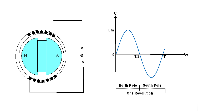 Figure 1 – Generation of Sinusoidal Voltage
The variation of the AC voltage magnitude (e) can be represented visually as shown in Figure 1. The voltage induced in the stator coil for one revolution corresponds to 1 cycle of the voltage as shown. For machines with more than two poles, one cycle corresponds to one pass of a pair of North-South poles.
Let us say one sinusoidal cycle (one revolution for a two-pole machine) corresponds to ‘T’ seconds. The number of cycles per second is defined as the frequency (f). The unit of frequency in SI units is a ‘Hertz (Hz). Once again, the SI unit of frequency or ‘cycles per second’ has been chosen in the honour of Heinrich Hertz, a German physicist. However, the unit ‘cycles per second’ is also popular in colloquial usage.
One cycle time ‘T’ is equal to (1/f ) seconds. Let us consider an AC system with a frequency of 50 Hz. The cycle time ‘T’ corresponds to 1/50th of a second or 20 milliseconds.
By plotting the sine curve of Figure 1 on a graph paper, we can read off the value of the voltage for a given time. However, the graphical representation has its own limitations. For example, if we wish to find the voltage at say, 2.532 seconds in a 50 Hz system, then we will need to plot the curve for a very long time. This is where mathematics comes to our rescue.
Sine Function
In mathematics, the sine (or cosine) function value for a given angle is obtained by means of a rotating vector (Em) as shown in Figure 2. The sine function for a given angle ‘θ’, is defined as the ratio of the vertical projection (AB) to the magnitude of the imaginary rotating vector (Em). In mathematics, a vector of unit length is commonly used for establishing the values of the sine function.
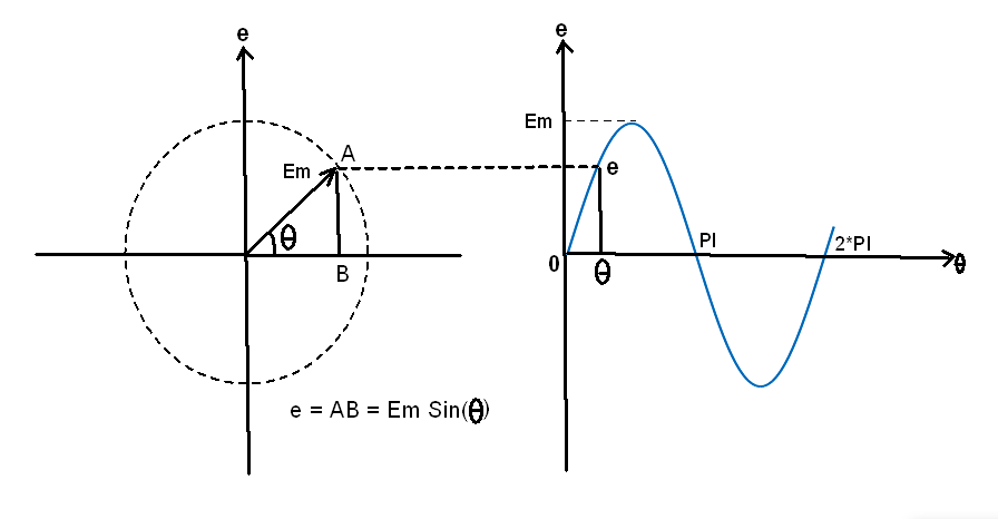
Figure 2 – Sinusoidal function
Using the sine function, we can write the equation for the sinusoidally varying voltage as given below.
e = Em sin(θ) … (1)
The value of angle ‘θ’ is normally expressed in radians or degrees. The SI unit for the angle is a ‘radian (rad)’. It is preferable to use the ‘radian’ for AC calculations, even though colloquially the popular unit is a ‘degree’.
The main issue with Equation 1 is that the voltage is expressed as a function of the angle ‘θ’. But, we need to express the AC voltage in Figure 1 as a function of ‘time’. Let us see how this can be done.
Representation of AC sinusoidal voltage
Referring to Figure 2, one revolution of the imaginary vector corresponds ‘2π’ radians, which corresponds to one cycle of the sinusoid. Referring to Figure 1, one cycle of the AC voltage (e) corresponds to a cycle time of T, which is equal to (1/f ) seconds.
Hence, one cycle time of (1/f ) seconds corresponds to one sinusoidal cycle of ‘2π’ radians. Therefore, the time (t) taken to travel an angle of ‘θ’ radians can be written as below.
t = [ θ / (2π) ] (1/f) seconds
or θ = (2πf)t radians
By substituting the value of θ as ‘2πft’ in Equation 1, we can write the equation for the sinusoidal variation of voltage at any given time as shown in Equation 2.
e = Em sin(2πf t) … (2)
where
e – voltage at any given time ‘t’ (volts)
Em – peak or the maximum voltage (volts)
f – frequency of the AC voltage (Hz)
The term ‘2πf’ in Equation 2 is traditionally replaced by the term ‘ω’, which is the angular velocity (radians per second) of the imaginary rotating vector (Em ) as shown in Figure 3.
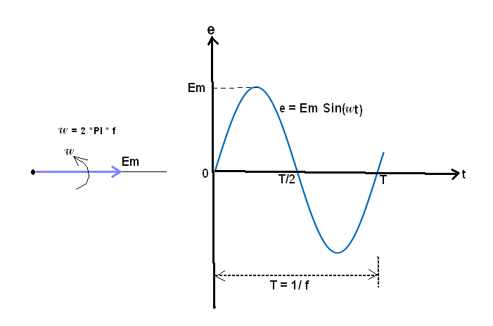
Figure 3 – AC voltage variation w.r.t. time
The product of angular velocity (ω) in ‘radians per second’ and the time (t) in ‘seconds’ results in the sinusoidal angle (θ) in radians! In the future, we will use the term ‘ω’ instead of ‘2πf’. The length of the rotating vector ‘Em’ corresponds to the peak magnitude of the AC voltage.
To be strictly mathematical, we must write ‘e’ as a function of time ‘e(t)’ in Equation 2. However, electrical engineers use lower-case letters such as, ‘e’ and ‘i’ to represent the time varying values, and upper-case letters such as, ‘E’ and ‘I’ for time invariant values.