
Electric Power – Part 3 – Reactive Power
Preamble
In the last blog (Electric Power – Part 2 – AC Power Concepts), we derived the equation for AC power as P = E I watts. This equation is valid only for pure resistive loads and it should NOT be used for general AC power calculations.
We shall derive a more general equation for AC power in a future blog. Firstly, we need to understand the power flow in AC circuits with inductances and capacitances. This in turn leads to the concept of ‘Reactive Power’ in AC circuits. The ‘Reactive Power’ is an important concept in AC power systems and is essential for the efficient operation of practical power systems.
It is important to remember the following factors regarding AC power calculations:
-
- The AC power (P) is the ‘Average Power’ over one cycle
- The actual instantaneous power (p) in AC varies with respect to time
- The voltage (E) and current (I) are ‘root mean square (rms)’ values
- The ‘rms’ value is given by Erms = Em / √2 and Irms = Im / √2
- The ‘rms’ value is a fictitious mathematical quantity
The ‘rms’ values are popularly used in AC systems to simplify power calculations. To make matters more confusing, the AC meters are designed to measure and display ‘rms’ values of voltages and currents. The corresponding physical quantity is the ‘peak or maximum’ value of the AC sinusoid. The peak values are rarely used in practice!
The ‘rms’ value is often referred to as the ‘equivalent DC’ value, since 1 ampere (rms AC) produces the same amount of heat as 1 ampere DC, when passed through the same resistance value.
Power flow in inductive loads
For pure inductance, the current flow in the inductance lags the corresponding voltage by 90 degrees. An inductance is a mathematical representation of the effect of magnetic flux (field) associated with electric circuits. The effect of the magnetic field is ignored in DC circuits since the DC magnetic flux does not vary with respect to time. However, in the case of AC, it cannot be ignored since the varying magnetic flux induces a voltage in the associated circuit element.
Let us now consider the power flow in inductive loads. A good example is an induction motor. An induction motor at rated load is mainly resistive – power corresponding to the mechanical load on the motor, but it requires an inductive current to produce the magnetic flux for motor action.
For an induction motor under rated load conditions, the current lags the voltage by a small angle ‘φ’. The vector diagram and the waveforms are as shown in Figure 1.
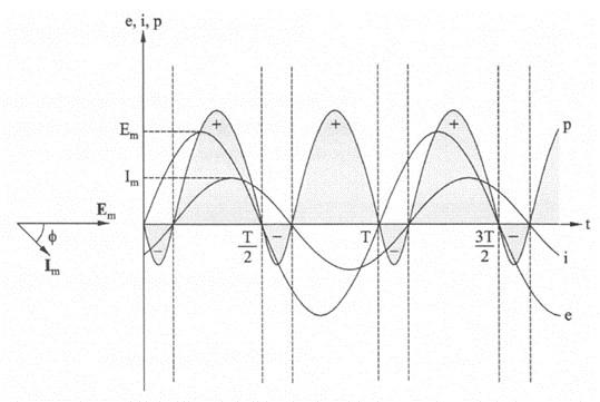
Figure 1 – Vector diagram and waveforms for a lagging load
The variation of the instantaneous power ‘p’ is as shown in Figure 1. It is obtained by multiplying the instantaneous values of voltage (e) and current (i) at a given instant of time.
It is interesting to note that the value of instantaneous power (p) is negative for some part of the cycle. What does this really mean?
As strange as it may sound, the power flows from the motor (load) back into the generator (source) when the power is negative! This reversal of power flow is due to the energy stored in the magnetic field (inductance) of the load. The inductance (magnetic field) does not consume any energy. The energy absorbed by the inductance is returned back to the source! In Figure 1, the positive (‘+’) part of the power cycle includes the energy absorbed by the inductance and the negative (‘-‘) part represents the energy returned to the source. The positive (‘+’) part of the cycle also includes the power consumed by the mechanical load, which is effectively a resistive load.
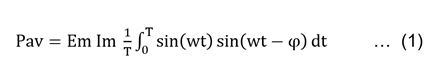
Let us write the equation for instantaneous power and calculate the average power using mathematics. We have,
e = Em sin(ωt)
i = Im sin(ωt – φ)
The equation for instantaneous power is as given below
p = e i
= Em sin(ωt) Im sin(ωt – φ)
We can calculate the average power (Pav) over one cycle as given below
 The evaluation of the Integral in Equation (1) is not for the faint hearted! During my teaching days, I used to give this as a homework problem!
The final result after the integration is as given below 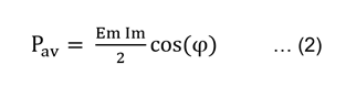 As before, we can replace the ‘Em’ and ‘Im’ by the corresponding root mean square (‘rms’) values, namely E = Em / √2 and I = Im / √2.
P = E I cos(φ) … (3)
Equation 3 is a general equation for ‘Average’ power for any given value of the phase angle ‘φ’. It is common to drop the subscript ‘av’ and use the symbol ‘P’. It is the power consumed by the load. Hence, we can say ‘useful’ power.
Equation 3 is also applicable for capacitive loads. However, the current leads the corresponding voltage vector in the case of capacitive loads.
In practical power systems, inductive loads are more common due to the extensive use of induction motors. In fact, almost 80-90% of the loads in practical power systems are induction motor loads. The rest are resistive loads, such as incandescent lamps and heaters. The capacitors are installed in power systems mainly to compensate for the large inductive loads.
Example 1
Calculate the average power flowing into the load for the following measured ‘rms’ values of voltages and currents. The voltage and currents are given as complex numbers with specified values of magnitude and angle.
Note: The bold font is used to represent the complex values and normal font is used to represent the magnitudes.
(a) V = 240 V @ 0o and I = 5 A @ -30o
(b) V = 240 V @ 0o and I = 5 A @ +30o
(c) V = 240 V @ 0o V and I = 5 A @ 0o
(d) V = 240 V @ -10o V and I = 5 A @ -30o
(e) V = 240 V @ 0o V and I = 5 A @ -125o
We have the equation for (average) power as given below
P = V I cos(φ) watts
where,
V – magnitude of the voltage (rms value)
I – magnitude of the current (rms value)
Φ – phase angle difference between voltage and current
(a) we have,
V = 240 V, I = 5 A
We are interested in the ‘phase difference’.
φ = 0o – (-30o) = +30o
The current lags the voltage. It is an inductive load.
P = V I cos(φ) = 240 x 5 x cos(30o) = 1039.23 watts
(b) we have,
V = 240 V, I = 5 A, φ = 0o – (+30o) = -30o
The current leads the voltage, it is a capacitive load.
P = V I cos(φ) = 240 x 5 x cos(-30o) = 1039.23 watts
(c) we have,
V = 240 V, I = 5 A, φ = 0o – (0o) = 0o
The voltage and current are in phase. It is a resistive load!
The phase angle difference is zero, but we can still use Equation 3.
P = V I cos(φ) = 240 x 5 x cos(0o) = 1200 watts
Note: For the same voltage and current magnitudes, a resistive load absorbs more average power! Hence, the power transfer is more efficient if the phase angle difference is close to zero. We are interested in this since we would like to operate the power system as efficiently as possible. We will discuss this in future blogs.
(d) we have,
V = 240 V @ -10o and I = 5 A @ -30o
We have an interesting situation now. This is a common occurrence in practice. The phase angle of the voltage at a given ‘reference’ node (bus) is assumed to be zero. All other bus voltage angles are expressed relative to the reference bus.
What is the phase angle difference for this case?
φ = -10o – (-30o) = +20o
A vector diagram shown in Figure 2 will help to visualise the phase difference.
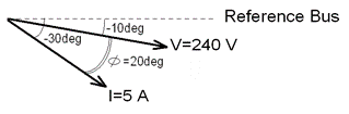
Figure 2 – Vector diagram
P = V I cos(φ) = 240 x 5 x cos(20o) = 1127.63 watts
Note that the current lags the voltage, therefore, this is an inductive load.
(e) we have,
V = 240 V @ 0o and I = 5 A @ -125o
The phase angle difference is
φ = 0o – (-125o) = +125o
P = V I cos(φ) = 240 x 5 x cos(125o) = -688.29 watts
What does the negative ‘average’ power mean? Confused? We will take a rain check for now and clarify it in the next blog!
Limitations of using P = E I Cos(φ)
Equation 3 is a popular equation for calculating power flow in AC circuits – especially in introductory courses on AC circuits. However, it has some limitations.
The main limitation of Equation 3 is that it does not quantify the oscillatory power flow as illustrated in Figure 1. For efficient operation of power systems, it is essential to keep the oscillatory flow to a minimum. Hence, the quantification of oscillatory power flow is an important first step for efficient operation of power systems.
It is preferable to have a power flow equation which calculates the phase angle difference automatically and also incorporates the significance of negative values of power.
Let us first consider the extreme case of oscillatory power flow before delving into quantification of oscillatory power flow.