
CT Specs – Part 4
Class PX and Differential Protection
Preamble
This is the final part in the series of blogs on current transformers. The topics covered in this blog are Class PX CT specifications. An understanding of Class PX specifications requires an appreciation of CT fundamentals and traditional differential protection concepts. Hence, an overview of both has been included in this blog.
The CT class designations PX, PS, PL and X are used in various CT standards. The good news is that all these standards have the same specifications. This blog focuses on Class PX specifications, however, it applies to the alternative designations.
This blog also presents an overview of differential protection using microprocessor-based relays and their effect on current transformer specifications.
CT Fundamentals
At the outset, it is important to note that the basic concepts for both Class P and Class PX type current transformers are the same. Let us recall the CT equivalent circuit developed in the blog on ‘CT Specs – Part 2 – Class P Application’. The CT equivalent circuit shown in Figure 1 is applicable for both Class P and Class PX.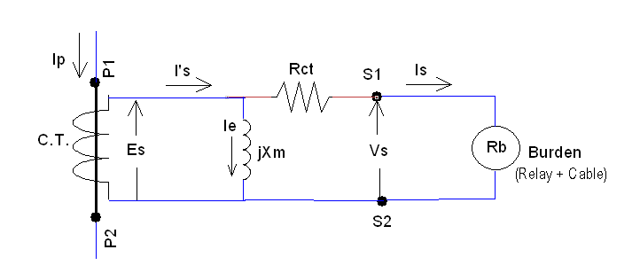
Figure 1. CT Equivalent Circuit
Equations used for the design of current transformers are based on Faraday’s law of induction, which is fundamental to electromagnetic phenomena.
e = N dφ/dt … (1)
where,
φ – Time varying flux at a given instant of time ‘t’ (Webers)
e – Induced voltage at that instant of time (Volts)
N – Number of turns in the coil (winding) which encloses the flux
In practice, we deal with alternating current (AC) systems, where the flux varies sinusoidally with respect to time at a fixed frequency. This is expressed mathematically as below:
φ = Φm sin (2πf t)
where,
φ – Magnetic flux at any given instant of time ‘t’ (Webers)
Φm – Maximum (Peak) value of the sinusoidal flux (Webers)
f – Frequency of the AC system (Hertz)
t – Time (seconds)
For a given magnetic path, we have:
Bm = Φm / A
where,
Bm – Maximum (Peak) value of the corresponding flux density (Tesla)
A – Area of cross-section of the magnetic path (square metres)
By substituting the above equations into Equation 1, we get the following:
e = N d [ Bm A sin(2πf t) ] /dt
= N A Bm (2πf) cos(2πf t)
For steady state conditions, the induced voltage (‘e’) will also vary sinusoidally. Note that the voltage leads the flux by 90 degrees.
The peak value of the voltage is obtained by ignoring the ‘cos(…)’ term. However, for practical calculations, we are interested in the ‘root mean square (rms)’ value of the voltage. Hence, we can write the simplified equation for the ‘rms’ value of the induced voltage (Es) as below:
Es = N A Bm 2πf / (√2 )
After simplification, we get the following equation:
Es = 4.44 f Bm N A volts … (2)
Equation 2 is the fundamental equation for transformer design – not just current transformers! In Equation 2, the induced voltage ‘Es’ is the ‘rms’ value and the flux density ‘Bm’ is the peak value! This is a quirk of mathematics and we are stuck with it!
For the sake of completeness, let us explore this topic a bit further. The relationship between the flux density (B) and the magnetising current (Ie) can be derived as detailed below.
The relation between the magnetic flux density (B) and the magnetic field strength (H) is as shown in Equation 3. Equation 4 is the Ampere’s law! This is the fundamental equation which relates the electromagnetic field and the electric field (electric current). Peak values have been used in Equation 3 and 4 for convenience. The equations are also valid for instantaneous and ‘rms’ values.
Bm = μ Hm … (3)
Hm = N Iem / l … (4)
where,
Bm – Peak flux density (Tesla)
Hm – Peak magnetic field strength (Amperes / metre)
μ – Permeability of the magnetic material (Tesla metre / Ampere)
N – Number of turns in the winding
Iem – Peak magnetising current (Amperes)
l – Length of the magnetic path (metres)
For a given electromagnetic system, the value of permeability (μ) is a constant, provided that the magnetic flux in the core is not saturated. This condition is true for most electromagnetic systems in practice. In such a case, we can combine Equations 2 to 4 and eliminate the magnetic quantities Bm and Hm. The resulting equation can then be expressed in terms of only electrical quantities, namely, voltage and current. The magnetic effect is then modelled by a constant value, namely ‘Inductance’ or ‘Inductive reactance’. In fact, the CT equivalent circuit shown in Figure 1 is based on this concept. It shows the induced voltage (Es), magnetising current (Ie) and inductive reactance (Xm). It does not make any reference to the magnetic field or the flux density!
The inductive reactance branch (Xm) shown in the CT equivalent circuit in Figure 1 is deceptive. The value of inductive reactance (Xm) is a constant only if the magnetic core is not saturated. Such an assumption is valid for voltage and power transformers, but it is not valid for current transformers. Current transformers are designed to saturate under fault conditions. The value of magnetising inductance (Xm) decreases dramatically when the CT core saturates. The magnetising branch (Xm) in the CT equivalent circuit is only decorative. We must use the CT characteristics provided by the manufacturer to establish the magnetising current (Ie) for a given value of induced voltage (Es) and vice versa.
Note: the subscript ‘m’ in ‘Xm’ denotes ‘magnetising’ reactance and it has no relevance to maximum (peak) value!
Very informative and clearly laid out. Thank you.
Thanks Alpana.
Regards,
Sesha
Hi
For clarity
The FIRST and FOREMOST criteria for diff prot is to make sure the relay will NOT OPERATE for a through fault even with one CT saturated.
That means you must get the the CT kneepoint Ek correct FIRST!
Assume CT2 is saturated.
Ek of CT1 must be at least sufficient to drive the secondary max fault current Ifmax through the saturated CT2
Ohm’s Law then says
Ek ≥ Is1max x (Rct1 + Rl1 + Rl2 + Rct2)
which simplifies to approximately
Ek ≥ 2 x Is1max x (Rct + Rl)
(you can see that the same equation applies for Ek of CT2 if CT1 is saturated)
Now we can consider the relay setting for that through fault condition where the relay MUST NOT operate!
Again, Ohm’s Law says if CT2 is saturated then the voltage at the relay is
Vs = Is1max x (Rl2 + Rct2)
So the effective relay setting Vr must be greater than Vs by a “margin”
If the relay is a voltage setting relay e.g. MFAC14, then the relay setting Vr must be greater than the calculated Vs.
No stabilising resistor is required as the relay is inherently a high impedance (MFAC14 operating current at any setting is ~20 mA).
If the relay is a current setting relay e.g. MCAG14 , then the relay setting is Id and we need the stabilising resistance.
The total minimum impedance is therefore
Rtot > Vs/Id
Rs = Rtot – Rrelay
If we assume the relay is zero impedance we can simplify to the correct version of Eq 8 as:
Rs > Vs/Id
It is just a Ohm’s Law mathematical coincidence that the Vr_minimum is half of the Ek_minimum
But it is not necessarily true that Vr_actual is half of Ek_actual
Hence Eq 8 is not truly correct that Rs is based on half the kneepoint voltage
The kneepoint voltage could be “5 times the minimum” which would result in a much larger than necessary Rs
That would mean the CT waveform for an internal fault is driven much harder and faster into saturation than necessary making it harder for the relay to operate.
It is really
Rs ≥ (Ek_min/2) / (Id)
I discuss this in my own technical reference site:
https://ideology.atlassian.net/l/c/6v3TpqKv
Hello Rod,
Thanks for your comments. I have updated the blog and included a note regarding the CT resistance.
Regards,
Sesha
I have to strongly disagree!
It is not feasible, and should not be done, to “specify Class P CTs for differential protection”
I agree that modern numerical relays provide some great features and settings that make things a lot easier.
Whilst the Ohm’s Law consideration of the CTs and settings for a Merz-Price Circulating Current High Impedance Differential do not apply in the same way to modern “low impedance relays” (i.e. relays with individual CT inputs not paralleled to the other CTs), the underlying principle of preventing unwanted diff relay operation for a through fault must still be applied.
That cannot be achieved by simply specifying P class CTs .
P class defines what you can connect to the CT in terms of total burden to achieve a certain accuracy at the ALF and rated burden.
PX class defines the construction of the CT to achieve a certain dynamic performance of a certain magnetisation curve and internal Rct.
You could have two CTs with the same P class specification but with VERY different Ek, Ie and Rct.
Consequently for the same through fault current connected to a very low burden such as a modern diff relay, at a particular “required” output current of the two CTs, the terminal voltage could be VERY different.
That means the Excitation current will be very different.
That means the real output current of each CT will be different … and that is not what we want fro a through fault as that means a false differential current calculation.
Yes, the relay settings MAY provide sufficient bias to compensate for differences of P class CTs.
But you have no idea what that difference is going to be when you specify P class CTs
You will ONLY know what the difference is when you test the actual P class CTs to determine their actual Ek, Ie and Rct
The real point of specifying PX is that we really need to know Vk, Ie and Rct anyway for diff applications and so we can ensure the dynamic performance based on the slope Vk/Ie is the same so that the “false differential current” is minimised
Hello Rod,
Thanks for your comments.
The aim of these blogs is to provide an in-depth exposure to CT fundamentals, theory and CT design. Based on the information provided, the protection engineer can make judicious decisions as per site requirements.
The motivation for including the Class P specifications for differential protection in this blog are as below:
1. The Schneider SEPAM manuals recommend the use of 5P20 Class P CTs for their microprocessor based differential protection. I have included a link to SEPAM manual information in this blog.
2. I had the personal experience of tailoring the Class P CT for differential protection. The site had specified and installed a 22kV Class P CT erroneously for transformer differential protection. This was discovered at the time of commissioning the project. Replacing the CT was not an option. I had to research the CT design details to tailor the Class P CT on the site for differential protection. Please refer to my blog on ‘CT Specifications – Gold Report’ for details.
Regards,
Sesha
Very informative
Rodney Huges response adds the value
Very detailed information, like the way it has been presented.
Easy to follow through with calculations.
Give a good insight on the IEEE & IEC CT sizing. Thank you.
You are welcome!