Electric Power – Part 2 – AC Power Concepts

Equation for power in AC systems

The equation for power in AC circuits at any given instant of time is as given in Equation 4.

                                    p  =  e x i                                … (4)

where,

                        p – power at any given instant time ‘t’  (watts)

                        e – voltage at time ‘t’  (volts)

                        i  – current at time ‘t’  (Amps)       

The above fundamental equation for electric power is valid at any given instant of time.  In fact, the above relation is valid for any variation, not just for sinusoidal AC.  However, in practice, the power calculations in AC systems are performed only for sinusoidal steady state conditions.

Note: Even when dealing with non-sinusoidal steady state conditions such as harmonic loads, it is a common practice to resolve the harmonic loads into sinusoidal components using transformation methods to perform the power calculations.

The value of power ‘p’ at any given instant of time ‘t’ is called the ‘Instantaneous power’.  This value obviously changes at every instant of time.  The instantaneous power is not of much use in practice for the design and operation of electrical equipment.  The value which is more useful is the ‘Average power’ for one cycle of sinusoidal variation. 

The ‘average power’ calculation for AC systems results in some interesting concepts which are fundamental to the design and operation of AC power systems.  Let us investigate these in the following sections.

Average AC power in resistive loads

This is the simplest case for average power calculation.  We know that the voltage and current are in phase for ‘pure’ resistance loads.  In practical AC power systems, the heater coils used in water heaters and space heaters can be considered as pure resistance loads.  Such loads are also called ‘unity’ power factor loads. (We will discuss the concept of power factor in detail in a future blog in this series). The phase angle between voltage and current is zero for unity power factor loads.

When the voltage and current are in phase, the waveforms for the voltage, current and power are as shown in Figure 4.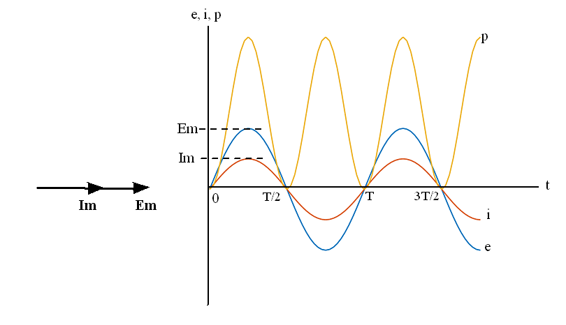

Figure 4 – Vector diagram and waveforms for unity power factor load

Using mathematical representation, we can write the equation for sinusoidal voltage and current at any given instant of time ‘t’ as below:

                                    e  = E_m sin(ωt)    

                                    i   =  I_m sin(ωt)

             where,

                        ω = 2πf   and   ‘f’ is the frequency of the wave in ‘Hertz’.

We can write the equation for instantaneous power as below,

                                    p  =  e  i

                                        =  E_m sin(ωt)  I_m sin(ωt)

                                        =  E_m I_m sin²(ωt)                                     … (5)

Note: As shown in Figure 4, the electric power output varies with respect to time.  Hence, the mechanical power applied to the rotor must also vary with respect to time.   For a good mechanical design, it is necessary to have a constant power operation, otherwise, the system will need a high-inertia flywheel.  This problem is solved in practice by using multi-phase AC machines.  We will discuss multi-phase systems in a future blog.

The area under the ‘p’ curve in Figure 4 indicates the energy.  Hence, the ‘Average power’ over one cycle is given by:

                      P_av = (Area under the ‘p’ curve for one cycle) / (Cycle time)

One can use the graphical methods to calculate the value of ‘P_av’.  However, the use of mathematics provides a more versatile and simpler result!  We can write the equation for ‘Average power’ mathematically as below.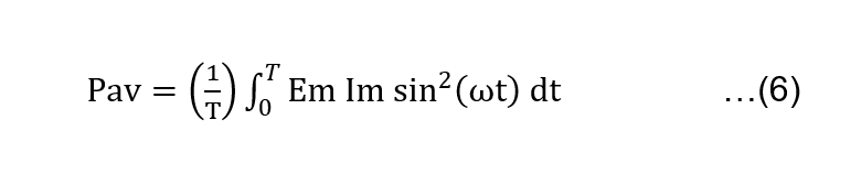

Even though evaluating the integral in Equation 6 is complex, the final result is surprisingly simple!  The result is shown is Equation 7.

                                    P_av = E_m I_m / 2                                   … (7)

Equation 7 can be re-organised further to get rid of the division by 2 in a very clever way! 

                                    P_av  =  (E_m / √2) (I_m / √2)  =  E_rms I_rms        … (8)

where,

                                    E_rms = E_m / √2     and    I_rms = I_m / √2

 The subscript ‘rms’ stands for the ‘root mean square’ value.  It is customary to use the ‘rms’ values when working with AC sinusoidal voltages and currents.  In fact, the use of ‘rms’ values in AC systems is so ubiquitous that, in practice, the values of AC voltages and currents are assumed to be ‘rms’ values unless otherwise specified.  Consequently, it is common to omit the explicit use of the subscript ‘rms’.  In addition, it is also common to drop the subscript ‘av’ for the average power ‘P_av’ 

Hence, the average power (P) in one cycle for resistive loads (voltage and current in phase) is written as below.

                                                P  =  E I  watts                                  … (9)

where

                        E  –  rms value of the voltage  (E_m / √2)

                        I   –  rms value of the current   (I_m / √2) 

Equation 9 for the average power over one cycle is identical to the equation for power in DC (Direct Current) system.  In fact, E_rms and I_rms are often referred to as equivalent DC values of voltage and current, respectively.